Describing Algorithms: Introduction
Denis Ignatovich
20 Jun 2019
•
9 min read

#Symbolic AI for algorithm state-space exploration
Our world runs on algorithms — from autopilot systems inside Boeing jets to “dark pools” run by investment banks to autonomous vehicle controllers. So it’s fairly important we understand how they might behave (especially when they can behave in ways we don’t want).
When describing an algorithm or a complex system, we often need to enumerate its “edge cases” or distinct behaviors, and illustrate them with concrete examples. The problem is that modern “real world” algorithms (systems) are designed to process (virtually) infinite collections of possible inputs (think of a Boeing autopilot system and the possible scenarios it can be in). So how do we manage this “infinity”?
At Imandra we’ve developed a technique for automatically describing and reasoning about algorithm state-spaces. We call it Region Decomposition and it is a core feature of Imandra, our cloud-native automated reasoning engine. It creates a quantitative ‘map’ of how a system might behave with sample points. One exciting application of Region Decomposition is for software testing as it creates a quantitative and explainable coverage metric of a system under test. In this post we’ll introduce Region Decomposition and outlines its many applications.

Intuition
The term Region Decomposition (RD) refers to a (geometrically inspired) “slicing” of an algorithm’s state-space into distinct regions where the behavior of the algorithm is invariant, i.e., where it behaves “the same.” Each “slice” or region of the state-space describes a family of inputs and the output of the algorithm upon them, both of which may be symbolic and represent many concrete instances. We’ll dive into examples below which will make everything clear, but for now remember this – each region of the state-space represents a “distinct” behavior of the system, and a decomposition is a collection of regions covering the entire space, including the so-called “edge-cases.”
RD is inspired by Cylindrical Algebraic Decomposition (CAD) but Imandra “lifts” these techniques to algorithms at large. There are many recent advances in formal verification, mathematics and computers science that are packed into Imandra to make this happen.
Describing algorithms’ behaviors this way has many exciting applications in automated software testing, reinforcement learning, autonomous systems and many other domains. In this and the subsequent posts we will go into more detail with examples and applications.
Let’s jump in and start to build the intuition!
Note: Imandra, our reasoning engine, supports OCaml and ReasonML at its lowest level (we’ll have Python interface out soon), so all of the examples presented here are in OCaml. Why OCaml (and ReasonML)? We’ve created a ‘mechanized formal semantics’ for the pure subset of OCaml which allows Imandra to automatically convert the code into axiomatic representation (i.e. mathematical logic) and reason about it similarly to how a mathematician would reason about a theorem. Since ReasonML is a syntactic extension to OCaml, we fully support it too.
Consider the following code fragment:
let g x =
  if x > 22 then 9
  else 100 + x

let f x =
  if x > 99 then
    100
  else if x < 70 && x > 23
  then 89 + x
  else if x > 20
  then g x + 20
  else if x > -2 then
    103
  else 99
;;
We have two functions g and f and the latter looks somewhat convoluted. (In OCaml, types are inferred from the code and since we’re using integer arithmetic operators and values, both x arguments in functions g and f are taken to be integers)
Function f takes x as input, which is an integer and there are quite a few integers, so how many distinct behaviors of f are there? Let’s ask Imandra!
When we run decompose command with the name of the function f, we get the following (we include a still screenshot below, but the full region decomposition can be interactively explored at try.imandra.ai):
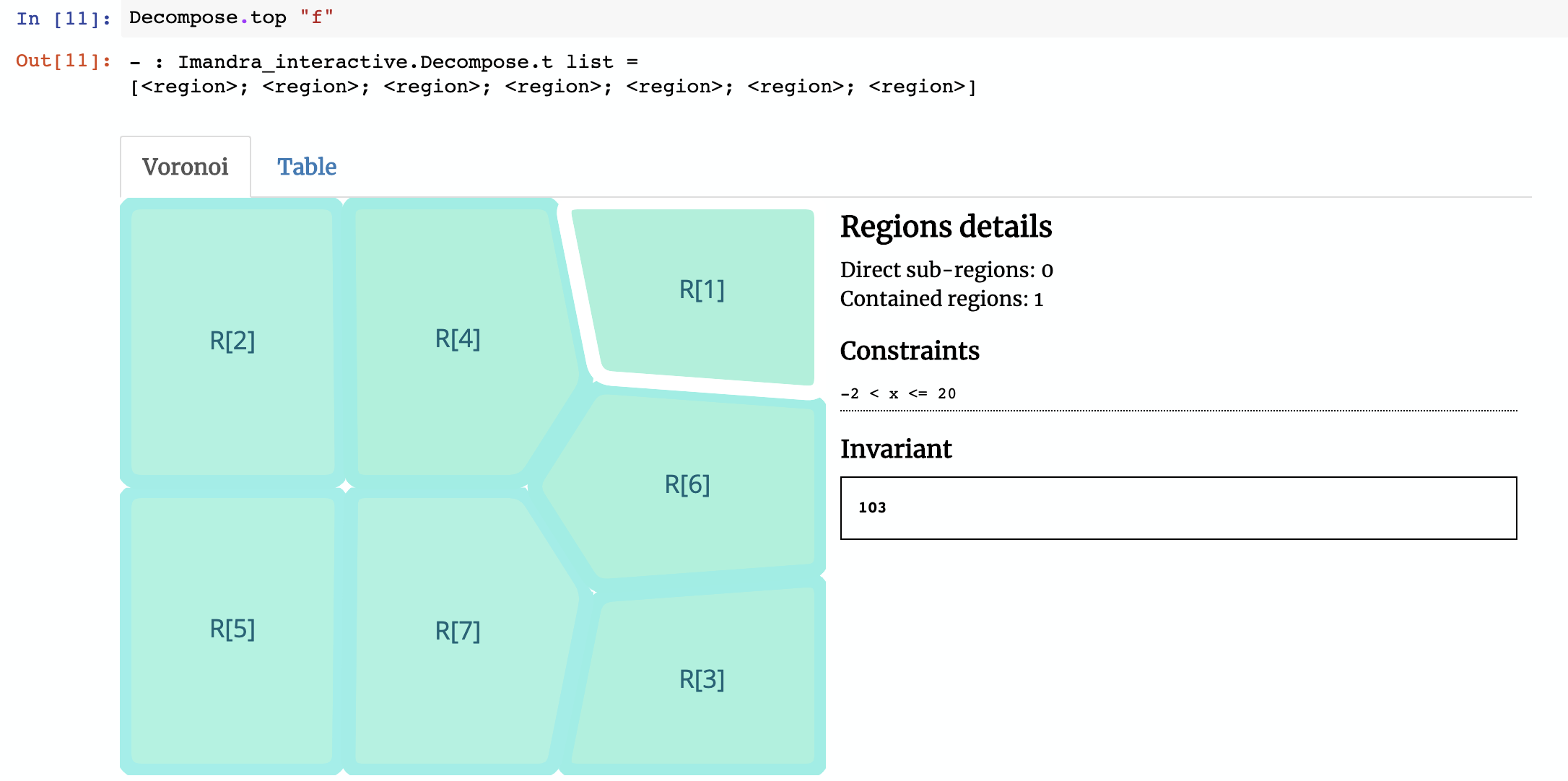
Imandra decomposes the function f into 7 regions. We’ve created a Voronoi widget for Jupyter Notebooks to help us visualize them. The region selected in the image above is R[1] (the naming convention refers to how Imandra decides to differentiate regions internally, based upon their symbolic relationships). In this decomposition, R[1] represents subset of the state-space where input x satisfies -2 < x <= 20 (e.g. -1 or 15) — in this region, the function will always return the value103. If you click on R[2], the constraint is 20 < x <= 22 and invariant result is x + 120. Notice that the invariant in R[2] is symbolic, so if x is 21 then the function will return 141.
If you combine all of these regions together, you will get the full behavior of f, a fact which Imandra mathematically proves behind the scenes.
Why RD scales
An immediate question might be whether RD scales to “real-world” algorithms. The answer is “Yes.” In fact, it is already deployed in production at some of the world’s leading financial institutions. It took us a few years of R&D and industrial POCs to get it right.
A naive approach would be to simply follow ‘branching’ within code and identify those paths as ‘distinct’ behaviors, but this would quickly ‘explode’ with even remotely complex algorithms. Moreover, when recursive functions are involved (even typical operations over Lists are recursive!), things get really tricky — Imandra is packed with quite a few powerful techniques to manage this.
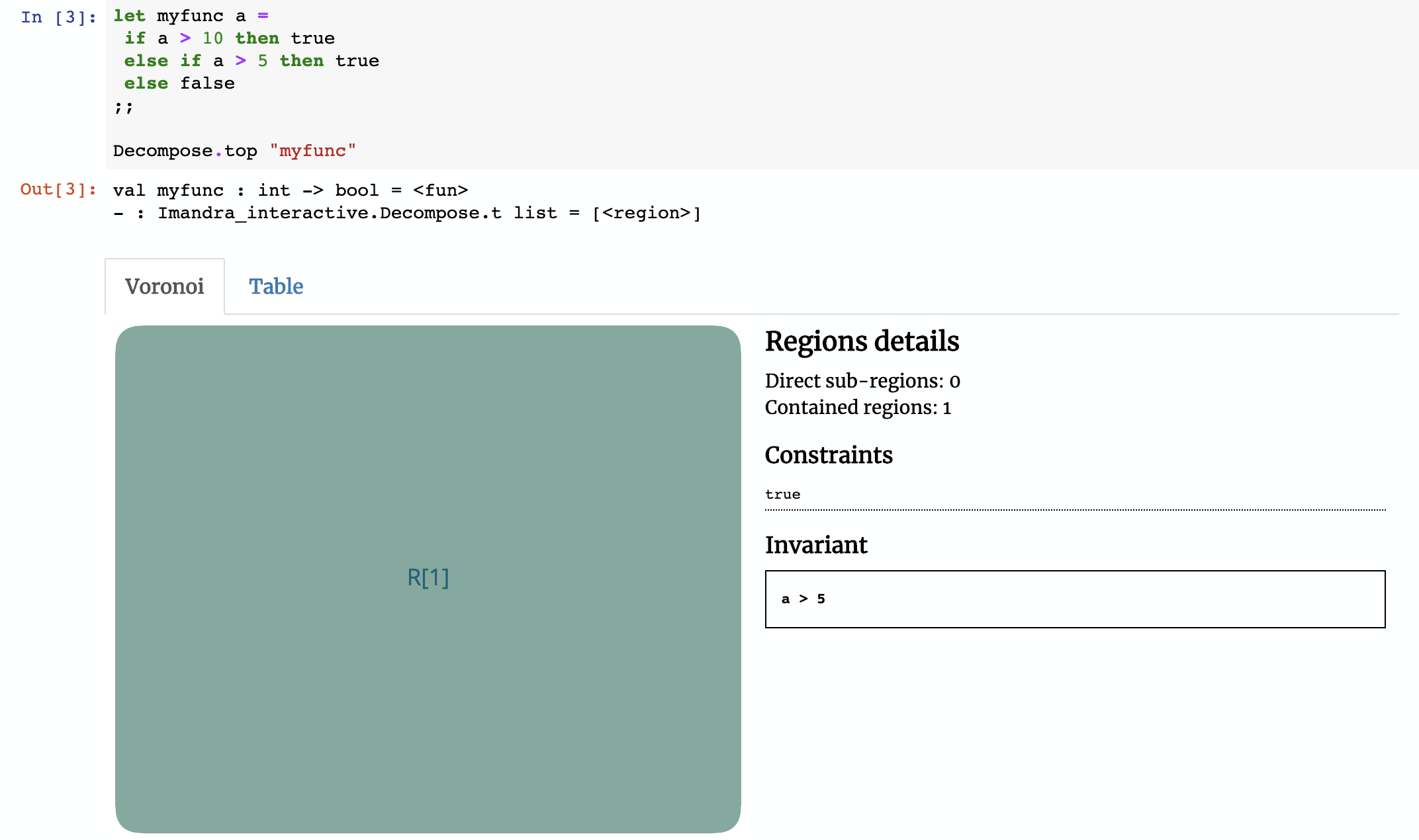
Here’s a small example to help illustrate how Region Decomposition works under the hood. Consider the function myfunc below:
let myfunc a =
 if a > 10 then true
 else if a > 5 then true
 else false
How many regions would you expect myfunc to have? The answer is 1 and if this wasn’t the case, then the approach we present here wouldn’t scale.
Imandra determined that myfunc may be described with a single region without any constraints on the input argument a and whose behavior is described by the invariant result of a > 5! For all possible values of a, the output of myfunc a is equal to a > 5, which of course could either be true or false.
Imandra’s support for Region Decomposition
As described, Region Decomposition is one of the core features of Imandra and there are quite a few ways you can use it.
At the lowest level (we have other front-end languages for RD including Python which we’ll cover later) Imandra accepts OCaml (and ReasonML). For the pure subsets of OCaml/ReasonML, Imandra (automatically) converts code into an axiomatic representation, applying numerous magical tricks and generating a state-space decomposition with an accompanying completeness proof. Each region in the decomposition also includes a solver which can be used to automatically generate inputs satisfying the region constraints. This feature is very useful for test-suite generation, for example.
In this section we’ll briefly cover transforming/printing regions into other formats (e.g. English prose) and using side-conditions to focus on various subsets of the algorithm state-space you’re decomposing. As always, please see our documentation at https://docs.imandra.ai for full information.

Transforms and printers
What can we do with these results? Well, since Imandra reflects the results back into the OCaml/ReasonML runtime, quite a lot:
-Synthesize inputs and test-cases: Given a region, we can ask Imandra to synthesize concrete inputs (as valid OCaml values) satisfying the region constraints. These are inputs which “push” the system into the given region. This provides a powerful basis for test-case and documentation generation, for example.
- Compute with them: From each region, an executable classification predicate can be automatically extracted, allowing you to take actual input values and figure out which regions they correspond to.
- Print/convert them into a format like FIX messages (used in finance)
We’ll look at an example of a printer for the longer example below.
Assumptions
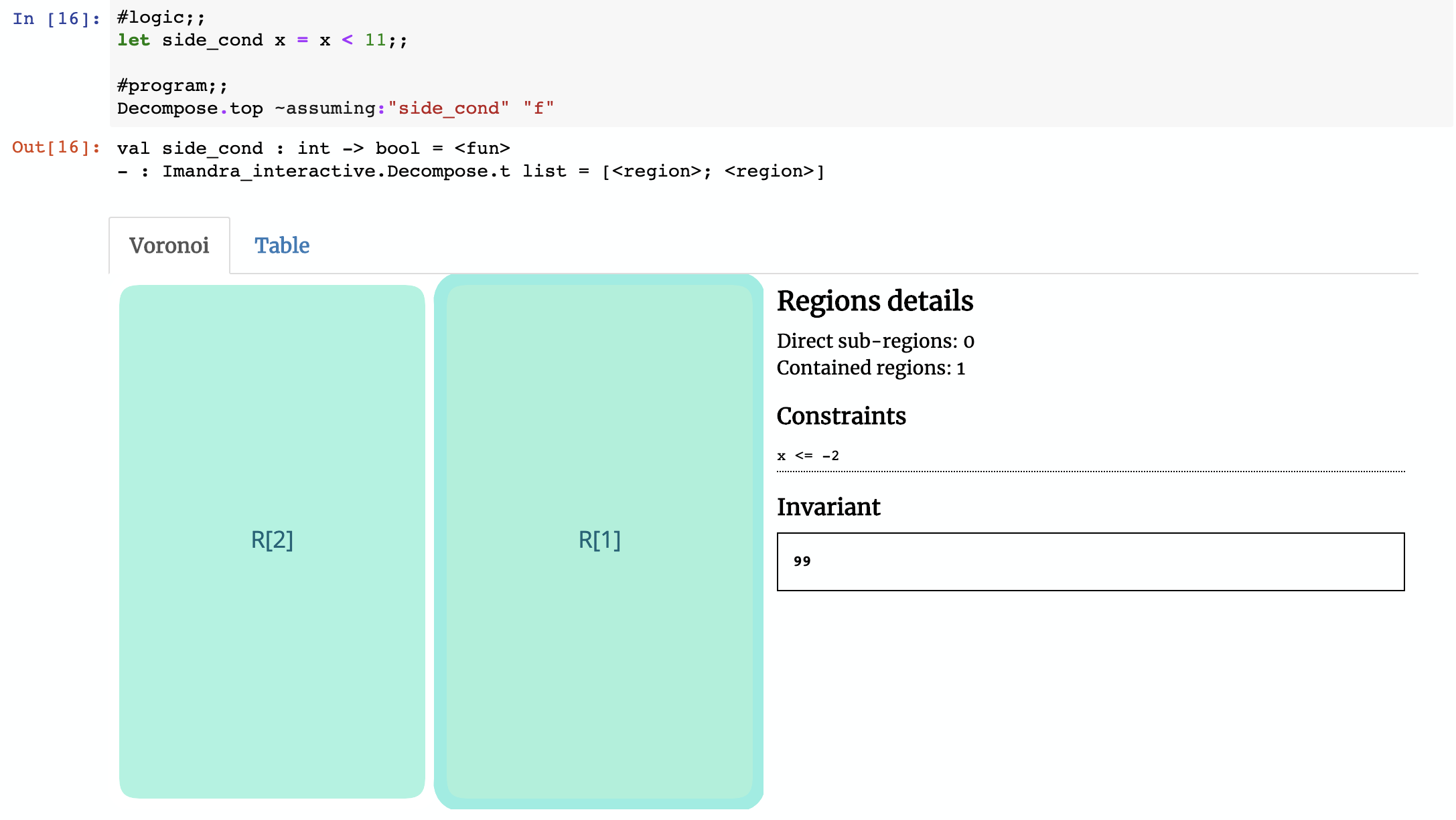
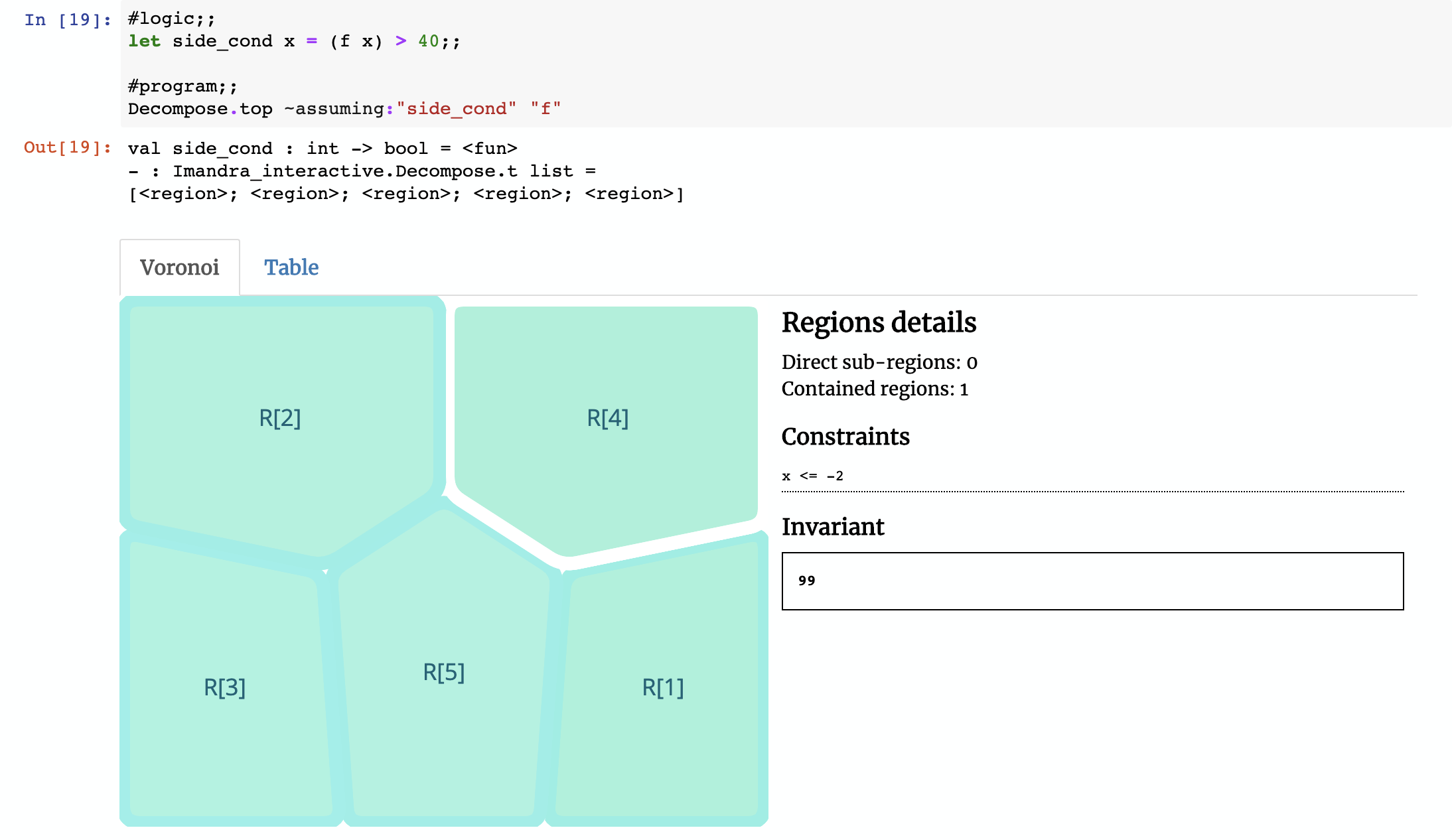
A key feature of Region Decomposition is the ability to superimpose constraints on the inputs and/or result of the function you’re decomposing. This allows you to focus on a specific subset of the state-space of the algorithm.
To to illustrate this, let’s revisit our first example function f. What if we wanted to restrict the input?
Since the side condition is just a boolean function, we can constrain the state space based on the result of running the function f:
Example: stock exchange pricing logic
Let’s now look at something a bit more complex and “real-world”. The complete example is in our documentation page (with a live Jupyter Notebook), so please check it out — we will just provide a high-level overview here.
Modeling financial venues with Imandra
Algorithms underpinning financial venues (exchanges and “dark pools”) are notoriously complex and are definitely “safety-critical”, so when they crash or ‘misbehave’, bad things happen. Naturally, they should be designed, tested and audited with formal methods. At Imandra, we’re making this a reality.
For this next example, we’re going to take a description of order book pricing logic from an actual exchange (SIX Swiss). This specific component determines the price of a transaction between a buy and a sell order, if the trade is possible. This logic would be just a fraction of the entire model of the exchange, but this is outside the scope of this exercise (interested readers should take a look at our white papers for complete discussion of how we model exchanges and other venues).
The main function of this code is as follows:
let match_price (ob : order_book) (ref_price : real) =
  (* Select the best buy and sell order of the order book (if they exist) *)
  let bb = best_buy ob in
  let bs = best_sell ob in
  match bb, bs with

  (* Now we'll match on values of `bb` and `bs`. We're using OCaml's option types -
  explicitly having a value of `None` when no `bb` or `bs` order exists. *)
  Some bb, Some bs ->
  begin
    match bb.order_type, bs.order_type with
    (* When we're matching Limit/Limit or Quote/Quote orders, then
        the outcome is simply limit price of the older order. *)
    | (Limit, Limit) | (Quote, Quote) -> Known (older_price bb bs)

    (* Logic gets more nuanced, however, when *)
    | (Market, Market) ->
      if bb.order_qty <> bs.order_qty then Unknown
      else
      (* need to look at other orders in the order book *)
        let bBid = match (next_buy ob) with
        Some bestBuy ->
          if bestBuy.order_type = Market then None
          else Some bestBuy.order_price
        | _ -> None in

        let bAsk = match (next_sell ob) with
        Some bestSell ->
          if bestSell.order_type = Market then None
          else Some bestSell.order_price
        | _ -> None in

      begin
        match bBid, bAsk with
        | (None, None) -> Known ref_price
        | (None, Some ask) ->
          if ask <. ref_price then Known ask
          else Known ref_price
        | (Some bid, None) ->
          if bid >. ref_price then Known bid
          else Known ref_price
        | (Some bid, Some ask) ->
          if bid >. ref_price then Known bid
          else
            if ask <. ref_price then Known ask
            else Known ref_price
      end

    | (Market, Limit) -> Known bs.order_price
    | (Limit, Market) -> Known bb.order_price

    | (Quote,  Limit) ->
      if bb.order_time > bs.order_time then
        (* incoming quote *)
        begin
          if bb.order_qty < bs.order_qty then Known bs.order_price
          else if bb.order_qty = bs.order_qty then
          match (next_sell ob) with
          | None -> Known bb.order_price
          | Some ord -> Known ord.order_price
          else Unknown
        end
      else
        (* existing quote's price is used *)
        Known bb.order_price

    | (Quote, Market) ->
      if bb.order_time > bs.order_time then
        (* incoming quote *)
        begin
          let nextSellLimit = next_sell ob in
          if bb.order_qty < bs.order_qty then Known bs.order_price
          else if bb.order_qty = bs.order_qty then
          match nextSellLimit with
          | None -> Known bb.order_price
          | Some ord -> Known ord.order_price
          else Unknown
        end
      else
        (* The quote's price is used *)
        Known bb.order_price

    | (Limit, Quote) ->
      if bb.order_time > bs.order_time then
        begin
          (* incoming quote *)
          if bs.order_qty < bb.order_qty then
            Known bb.order_price
          else
            if bb.order_qty = bs.order_qty then
              match (next_buy ob) with
              | None -> Known bs.order_price
              | Some ord  -> Known ord.order_price
            else
              Unknown
        end
      else
        (* existing quote's price is used *)
        Known bs.order_price

    | (Market, Quote) ->
      if bb.order_time > bs.order_time then
        begin
          (* incoming quote *)
          if bs.order_qty < bb.order_qty then Known bb.order_price
          else if bb.order_qty = bs.order_qty then
          (match (next_buy ob) with
          | None      -> Known bs.order_price
          | Some ord  -> Known ord.order_price
          )
          else Unknown
        end
      else
        (* The quote's price is used *)
        Known bs.order_price
      end
    | _ -> Unknown
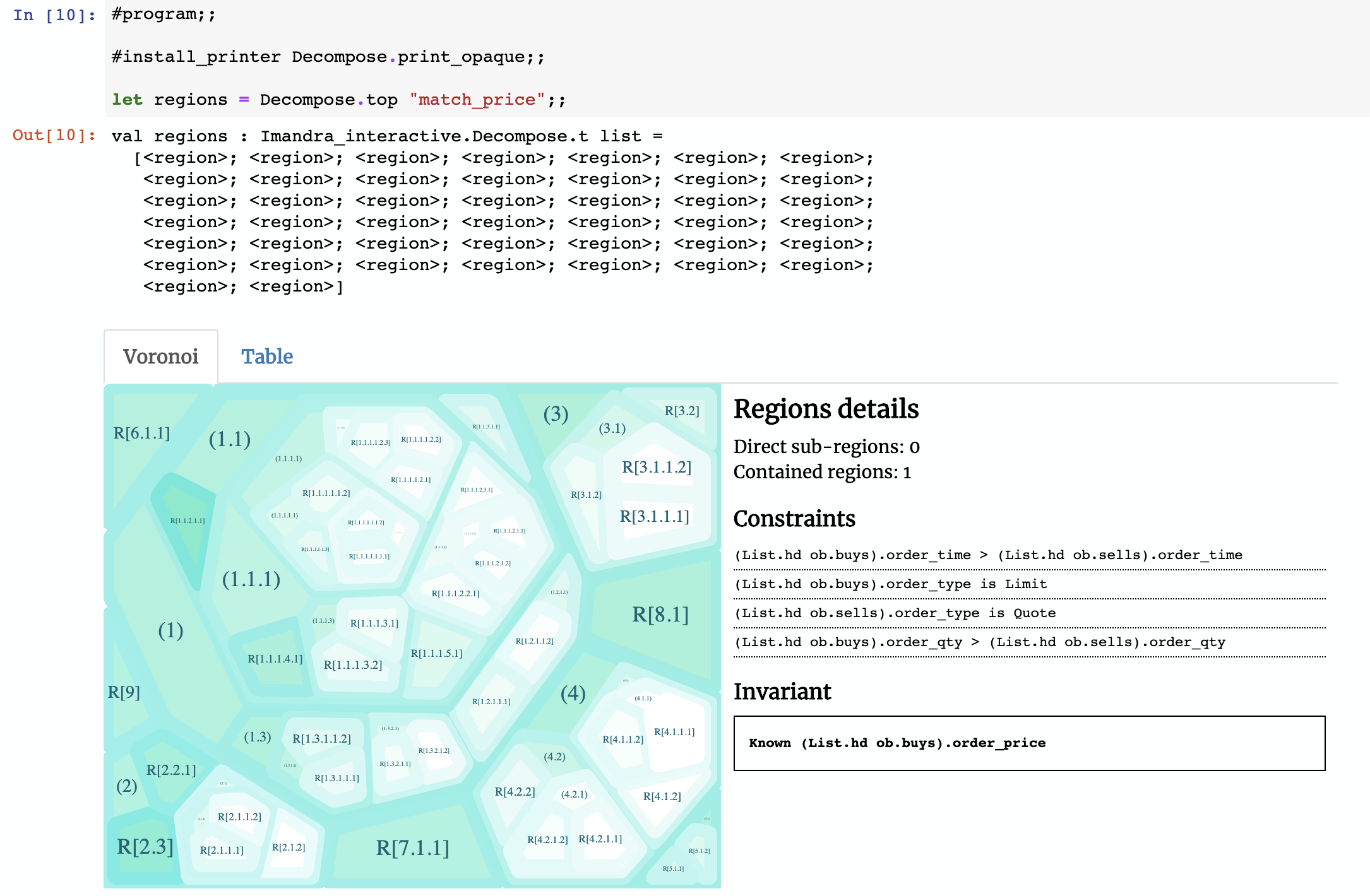
When we ask Imandra to decompose this function, we get this:
Writing custom printers
The constraints as they’re written by default are basically OCaml – you’ll notice some of the constraints contain List.hd ob.buys or List.hd ob.sells. Those are references to the first buy and sells orders using the standard OCaml list functions. To make this more readable we can make use of OCaml’s pattern matching and Imandra’s extensibility to create a custom printer (the notebook has full source code):
module Refiner = struct
 open PPrinter

 let walk (x : node) : node = match x with
  | Funcall ("List.hd", [FieldOf (_, "buys", _)]) -> Var "First buy order"
  | Funcall ("List.hd", [FieldOf (_, "sells", _)]) -> Var "First sell order"
  | Funcall ("List.hd", [Funcall ("List.tl", [FieldOf (_, "buys", _)])]) -> Var "Second buy order"
  | Funcall ("List.hd", [Funcall ("List.tl", [FieldOf (_, "sells", _)])]) -> Var "Second sell order"
  | Is (t, ty, FieldOf (_, "order_type", x)) -> Is (t, ty, x)
  | FieldOf (Assoc, (("order_id" | "order_qty" | "order_price" | "order_time") as field), x)
    -> FieldOf(Human, field, x)
  | x -> x

 let refine node =
  XF.walk_fix walk node
   |> CCList.return
end
After we install this new printer and view the regions, we see the constraints printed in a much more ‘human-readable’ format (if you spend more time on the printer, you can do much more!).
It’s a pretty powerful technique — we’ve gone from a pure executable OCaml algorithm describing the business logic (a simulator) to automated generation of edge case descriptions in English-like prose!
Generating test cases
The last step we’ll perform is generating sample points for the regions. A natural use case for these samples are test cases. Imagine you create a model of the system you would like to test and ask Imandra to describe its regions (or ‘edge cases’) and construct inputs for each one of them. This will give you test cases and also a quantitative coverage metric describing what it is that you’re actually testing!
What’s next
In this post, we have introduced Region Decomposition — a powerful technique of describing algorithm state-spaces. The next posts in this series will cover more advanced features and applications. Here’s the current plan:
- Describing Algorithms: Iterative Decomposition Framework (IDF) — a powerful Imandra toolkit for cloud-native parallel decomposition and reachability.
- Describing Algorithms: Reinforcement Learning — application of Region Decomposition to improving training of reinforcement learning algorithms.
- Describing Algorithms: Verified Autonomy – will discuss application algorithm state-space decomposition to certifying autonomous vehicles.
- Describing Algorithms: Decomposition Flags - covers the available options for performing Region Decomposition.
- Describing Algorithms: Transformers and Printers – demonstrates the pipeline you can use for region transformers and custom printers.
If you have any questions or requests, don’t hesitate to drop us a line (or two) in our Discord server.
Stay tuned!

WorksHub
Jobs
Locations
Articles
Ground Floor, Verse Building, 18 Brunswick Place, London, N1 6DZ
108 E 16th Street, New York, NY 10003
Subscribe to our newsletter
Join over 111,000 others and get access to exclusive content, job opportunities and more!